Optimization is an essential part of training deep learning models. Basically, it is a vital part of learning even by humans. Let’s consider a newborn baby, when you ask the baby a question he doesn’t know what to reply with, show the baby an object he does not know, why? His brain is still fresh and blanks with no data present.
So how does he become smarter over time and intelligent? He has to undergo a dynamic learning process, also while learning how sure is he about what he has learned? He has to be penalized on wrong deeds and praised for good deeds, exactly how the machine learns. So in deep learning tasks, we design neural network architectures with some initialized parameters known as weight and biases, then compile the architecture to make a model that knows nothing.
How do we teach the model?
After designing the model, we pass in some training features say x, and get an output y
i.e y = M(x), where M is the model, x is the input, and y is the output. The output y we got would still be very incorrect, to determine the magnitude of the incorrectness, we apply a loss function to the output to calculate how far it is from the true answer, i.e L(y, y’), this is where optimization comes in. Also, note that the loss function is a differential function with respect to the model parameters.
What is optimization
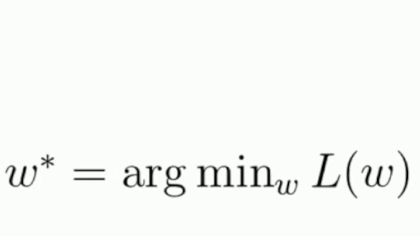
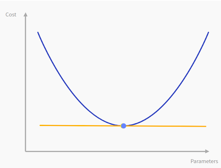
Optimization is basically the technique of reducing the loss of a model’s output, by taking gradient steps (gradient descent) to find the minimum loss that gives the optimum accuracy. We take the derivative of the loss with respect to the model parameter and modify the parameters in direction of decreasing loss.


Optimization techniques:
- Gradient Descent: This method iteratively steps in the direction of the negative gradient to get the lowest loss over the entire training set. However, this approach isn’t good enough as the model as to wait for a longer period of time to run the gradient descent algorithm on the entire data. This now leads to the development of a new technique known as STOCHASTIC GRADIENT DESCENT.

- Stochastic Gradient Descent: Instead of taking the gradient changes over the entire training set, we compute derivatives on batches of the training set and update the parameters over each batch. Examples of the batch size used are 32, 64, 128 e.t.c

Hyperparameters for SGD are Learning rate, batch size.
Learning rate is a really important parameter for optimization because it helps to determine the magnitude of steps we would be taking, either high or low. Consider this below:
dL\dw = wi
w = w- w’,
if the new weight is reset to the new derivative, it may cause high steps downward causing it to miss some important steps, so to reduce the step we multiply the new weight with a hyperparameter known as learning rate (LR). Therefore W = w- wi * LR, LR should be a small value below 1 i.e 0.1, 0.01,0.x…
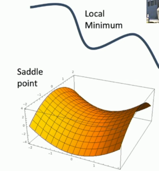
SGD face some problem which doesn’t cause the parameters to be optimized effectively, i.e. saddle point or local minimum, a point that has zero gradients but isn’t that actual minimum. This now led us to another version of SGD known as SGD+Momentum

- SGD + Momentum: This is the same as SGD, just that it has another hyperparameter that controls the energy required to overcome saddle points. The hyperparameter is known as ‘Rho’ and its default is 0.9. It computes the velocity at the time (t), starting with initial velocity zero, it takes gradients too.
V = 0
wi = dl/dw
v = rho * v + wi
w = w – v*lr
- AdaGrad: This also helps to modify SGD, not with momentum, but with the square of the gradient.
sqr_grad = 0
wi = dl/dw
sqr_grad = sqr_grad + (wi)2
w = w – (wi*lr) / sqrgrad+ 1e-7
- RMSProp: This is basically tweaking the AdaGrad algorithm by adding a decay rate to the square of the computed gradient.
sqr_grad = 0
wi = dl/dw
sqr_grad = decay_rate * sqr_grad + (1- decay_rate) + (wi)2
w = w – (wi*lr) / sqrgrad+ 1e-7
Hyperparameters for RMSProp are: Learning rate, decay_rate.
- ADAM: This called Adaptive momentum, it implements RMSProp + momentum
moment1 = 0
moment2 = 0
wi = dl/dw
moment1 = beta1 * moment1 + (1- beta1) * (wi)
moment2 = beta2 * moment2 + (1- beta2) * (wi)2
w = w – (moment1*lr) /moment2+ 1e-7
Hyperparameters for ADAM are: Learning rate, beta1, beta2.
Takeaway: ADAM is very good to start with as an optimizer, with beta1 = 0.9, beta2 = 0.999, learning_rate:[1e-3, 1e-4, 5e-4]

